Preparation for Simplex Method With Python

Before we go to the simplex method, we need to learn how to represent the linear program in an **equational form **and** **what are **basic feasible solutions**.

Equational Form

The simplex method requires an equational form of linear program representation. It looks like this:

Maximize cᵀx subject to Ax=b, x≥0

x is the vector of variables, A is a given m×n matrix, c∈ Rⁿ, b∈ Rᵐ are given vectors, and 0 is the zero vector, in this case with n components. All variables in the equational form have to satisfy the nonnegativity constraints.

Transform to equational form

Let’s grab the linear program from the previous part and represent it in equational form.

Maximize the value x₁ + x₂ among all vector (x₁, x₂) ∈ R², satisfying the constraints:
  x₁ ≥ 0
  x₂ ≥ 0
  4x₂ - x₁ ≤ 13
  x₂ + 2x₁ ≤ 10

1. In order to convert the inequality 4x₂ -x₁ ≤ 13 we introduce a new variable x₃, together with the nonnegativity constraint x₃ ≥ 0, and we replace the considered inequality by the equation -x₁ + 4x₂ + x₃ = 13. The additional variable(slack variable) x₃, which won’t appear anywhere else in the transformed linear program, represents the difference between the right-hand side and the left-hand side of the inequality.

2. We need to do the same with x₂ + 2x₁≤ 10. We introduce a new slack variable x₃, together with the nonnegativity constraint x₄ ≥ 0. As a result, we have this equation 2x₁ + x₂ + x₄ = 10.

3. The resulting equational form of our linear program looks this way:

Maximize x₁ + x₂ subject to
  -x₁ + 4x₂ + x₃ = 13
  2x₁ +x₂ + x₄ = 10
  x₁ ≥ 0, x₂ ≥ 0, x₃ ≥ 0, x₄ ≥ 0

Geometry

As is derived in linear algebra, the set of all solutions of the system Ax = b is an affine subspace F of the space Rⁿ. Hence the set of all feasible solutions of the linear program is the intersection of F with the nonnegative orthant, which is the set of all points in Rⁿ with all coordinates nonnegative.

2D

Let’s come back to the previous example. We have two equations that describe lines. In such case after solving system, we will obtain the only solution — point.

Let’s take a look at another example.

Maximize x₁ + x₂ subject to
  x₁ + x₂ = 3
  x₁ ≥ 0, x₂ ≥ 0

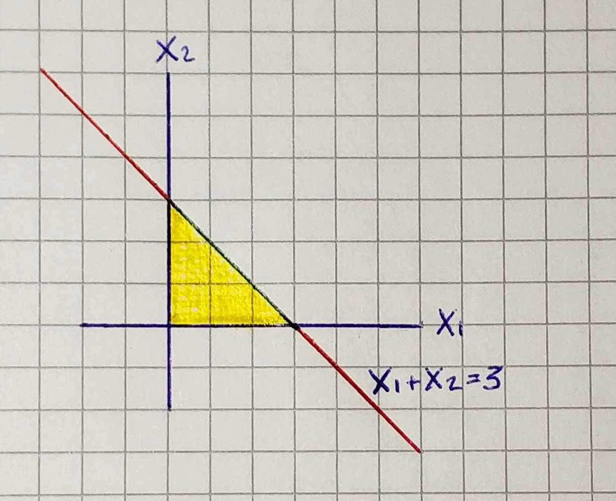
In this linear program we have only one equation and therefore the set of all solutions — line(red) and the set of all feasible solutions — segment(green).

3D

If we have n=3 variables and m=1 equation, for example x₁ + x₂ + x₃ = 3 we will have this picture:

The set of all possible solutions of Ax = b in this example is a plane. If we apply nonnegativity rule(*x₁ ≥ 0, x₂ ≥ 0, *x₃ ≥ 0), we will obtain the set of all feasible solutions(orange triangle).

With an understanding of what is the equational form, we can state the requirements for a linear program.

We will consider only linear program in equational form such that
1. The system of equations Ax=b has at least one solution.
2. The rows of the matrix A are linearly independent.

If the system Ax = b has no solution linear program has no feasible solution either. If some row of A is a linear combination of the other rows, then the corresponding equation is redundant and it can be deleted from the system without changing the set of equations.

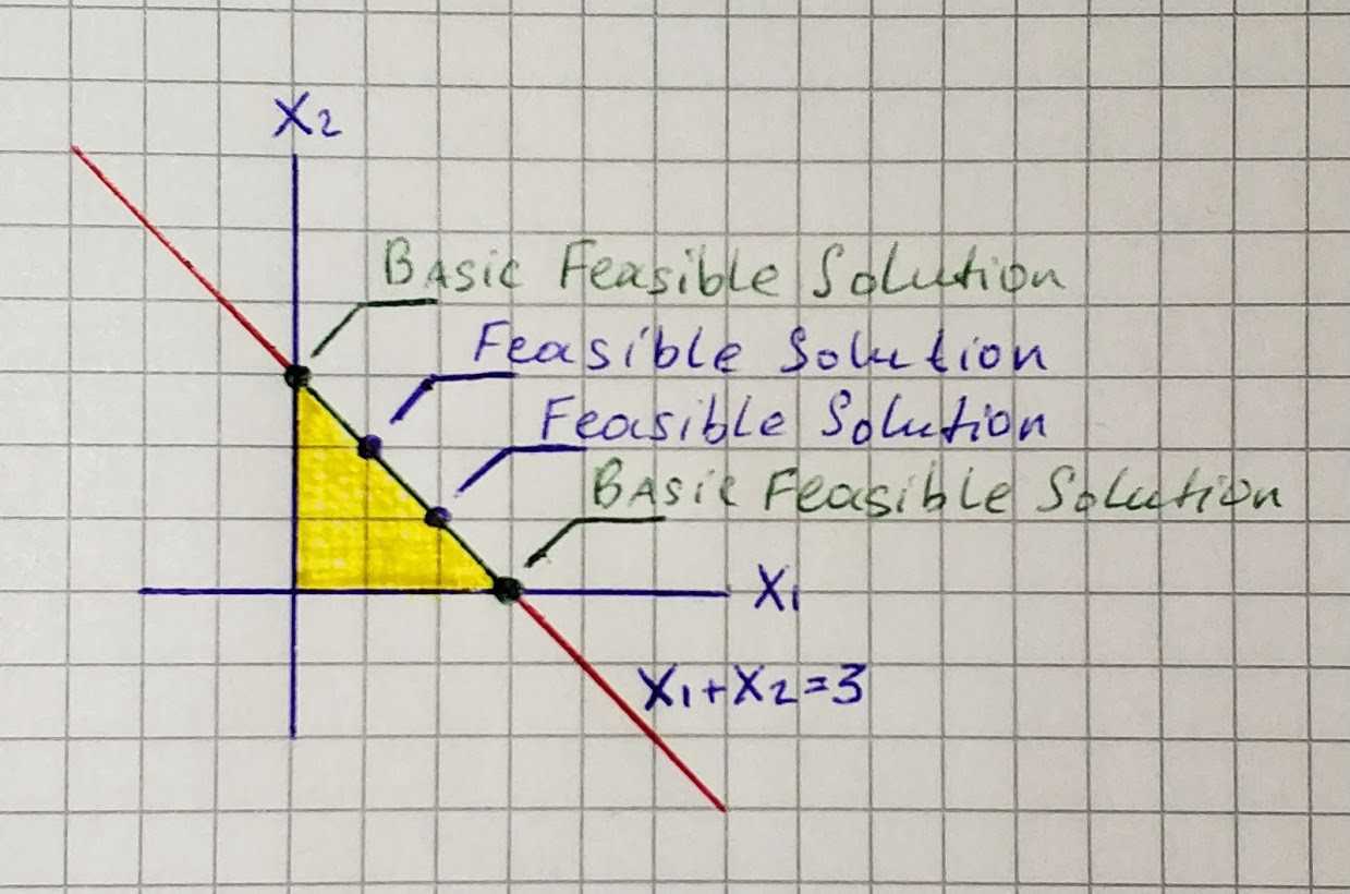
Basic Feasible Solutions

Among all feasible solutions of a linear program, a privileged status is granted to basic feasible solutions. Expressed geometrically a basic feasible solution is a tip (corner, spike) of the set of feasible solutions.

A basic feasible solution of the linear program
    maximize cᵀx subject to Ax=b, x≥0
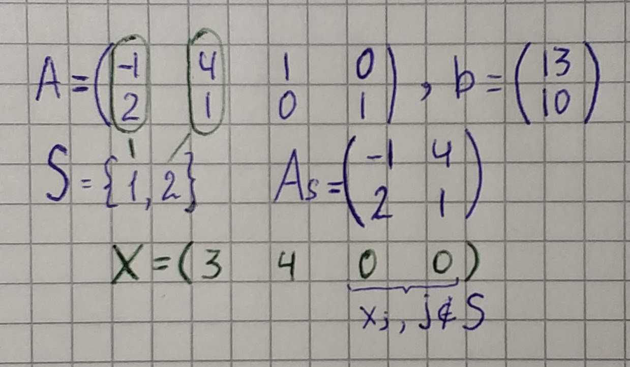
is a feasible solution x∈ Rⁿ for which there exists an m-element set S *⊆ {1, 2, . . . , n} such that
1. The (square) matrix Aₛ is nonsingular, i.e., the columns indexed by B are linearly independent.
2. xⱼ=0 for all J ∉ S.

If such a S is fixed, we call the variables xⱼ with* j ∈ S* the basic variables, while the remaining variables are called nonbasic.